It's All About the Base(line)

Climate fueled extreme weather, Part 5

Pulling the strings

This is Part 5 in the THB series — Climate Fueled Extreme Weather. You can find Part 1 here, Part 2 here, Part 3 here, and Part 4 here. Each can be read on their own, but I encourage you to start from the beginning as each installment draws on the ones before. If you have made it this far that you know what the IPCC really says about extreme weather and climate change.

Let’s start Part 5 with the conventional wisdom:

• A frequently cited climate scientist: “We know what to do – stop burning fossil fuels and replace them with more sustainable, renewable sources of energy. Until we do that, extreme weather events intensified by climate change will continue to destroy lives and livelihoods.”

• The Guardian (U.K.): “Emissions must plummet to stop extreme weather from growing more violent.”

• U.S. National Public Radio: “With tens of thousands of people displaced by floods, wildfires and hurricanes this summer, researchers warn that the majority of untapped fossil fuels must remain in the ground to avoid even more extreme weather.”

Can our decisions about energy can stop or reduce extreme weather?

The answer is no — and you won’t have to just take my word for it. In this post, Part 5 in the series, I review what the Intergovernmental Panel on Climate Change (IPCC) says about detecting and influencing changes in extreme events from the different baselines that it uses to assess change.

Parts 3 and 4 of this series discussed the concept of “time of emergence” which is when the signal of a change in climate for a particular metric is detectable in the context of internal variability of the climate system. The IPCC has been consistently explicit about the challenges of achieving detection not just in metrics associated with extreme events, but for other variables as well.

For example, the IPCC figure below shows an envelope of model projections (specifically, 100 RCP4.5 simulations using the MPIS ESM Grand Ensemble) for four different variables: ocean heat content, global surface temperatures, UK summer temperature, annual Arctic sea ice volume, and September Arctic sea ice extent.¹

Source: IPCC AR6 WG1 Chapter 1.

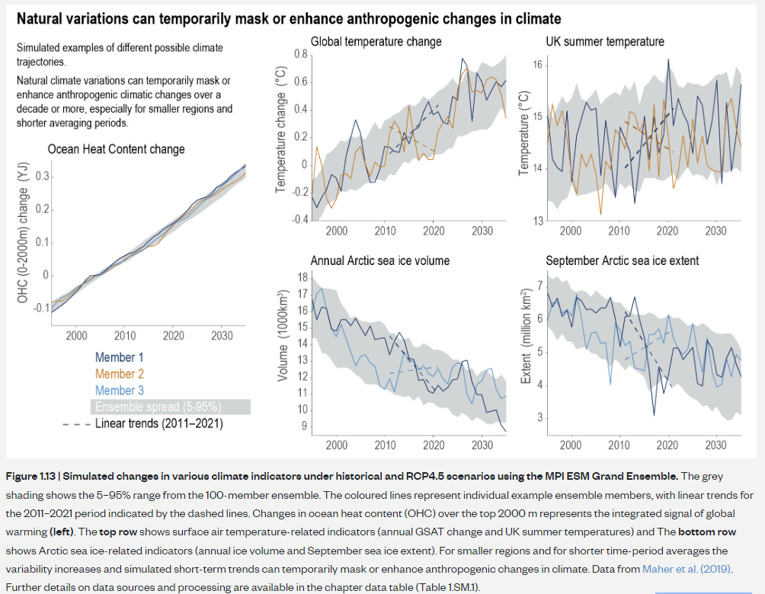
With the exception of ocean heat content, individual model realizations for the other four variables show considerable variability on decadal and multi-decadal time scales, such that even when climate is changing, over decades we can see both up and down trends in these metrics.²

The IPCC explains of the figure:

[F]or a representative 11-year period, both positive and negative trends can be found in all these surface indicators, even though the long-term trend is for increasing temperatures and decreasing sea ice. Periods in which the long-term trend is substantially masked or enhanced for more than 20 years are also visible in these regional examples. This highlights the fact that observations are expected to exhibit short-term trends which are larger or smaller than the long-term trend or that differ from the average projected trend from climate models, especially on continental spatial scales or smaller.

Importantly, note that ocean heat content does not exhibit large variability. That is why Roger Pielke Sr. (and others) have long advocated the use of ocean heat content as the primary metric to detect the warming of the climate system.

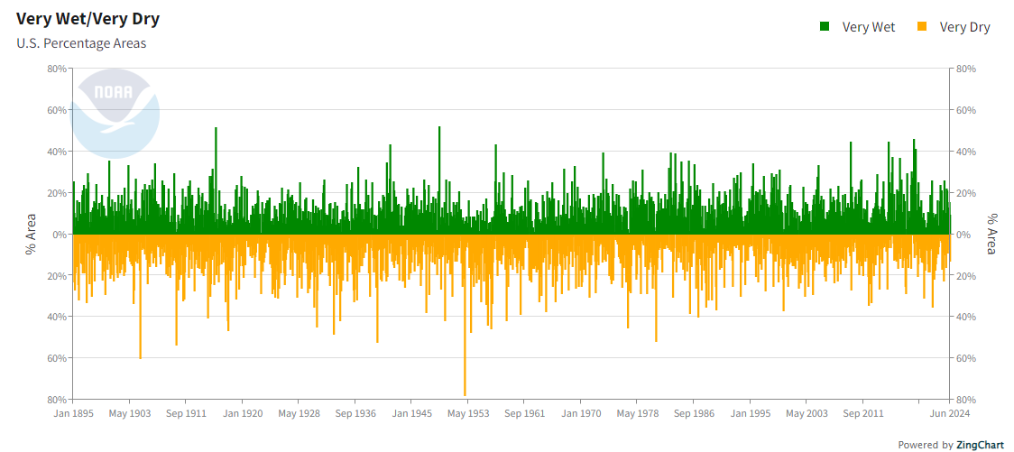
Time series of metrics related to extreme events can be much more variable that those examples above highlighted by the IPCC. Consider the percentage of the continuous United States in either very dry or very wet conditions, as shown below. Good luck detecting anytime soon a projected century-long change of a few percent up or down.

Source: NOAA

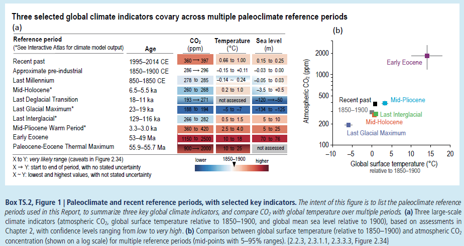
The IPCC explains that a change in climate refers to a change in the statistics of weather with respect to some baseline period. For purposes of detection and attribution of change, the IPCC uses two baselines: 1850-1900 (“approximate pre-industrial”) and 1995-2014 (“recent past”).³ The IPCC also uses scenario-based projections as a counterfactual baseline against which to assess the impacts of mitigation policy on specific climate variables — This is how we would assess whether climate policy might affect the weather we see outside our windows.

Detection of changes in climate variables is much more difficult to achieve with respect to the recent past (1995-2014) than further back in time because only a decade has passed since that period. Expected change from the recent past is much more meaningful to people and infrastructure than from pre-1900. That said, ecosystems that have evolved over centuries and longer may be more affected by changes that occur over longer time scales. Both baselines are thus important.

In Part 1 of this series I introduced a thought experiment:

Imagine that you are dealt two cards from a standard combined blackjack deck of 6x52 cards (that is, six combined 52-card decks). From this combined deck, the chances of being dealt at least one ace in a two-card hand is about 14.8%.⁴

Every ace added to the deck increases the odds of receiving at least one ace in a two-card hand by about 4%. For comparison, in 2020 the World Meteorological Organization reviewed published studies and suggested that globally, the most intense tropical cyclones (Category 4-5) would decrease in frequency by 2100 by about 3% and increase in intensity by about 5%.⁵

With one added ace, it would take 329 two-card hands to reach the IPCC’s threshold for detection of change in the combined deck.

What about the situation where we do not know if the deck has been stacked or how many additional aces have been added? In this situation, change is not assumed, but instead must be detected.

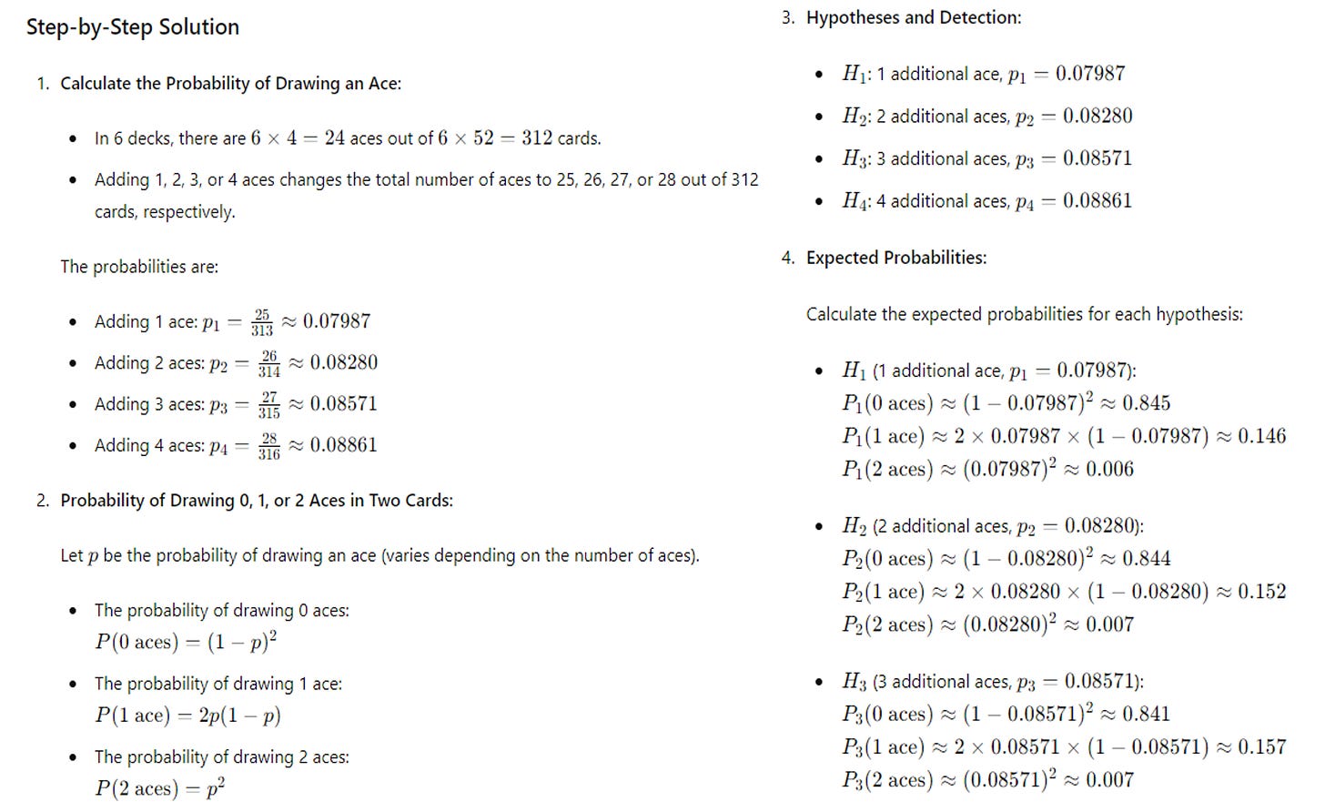
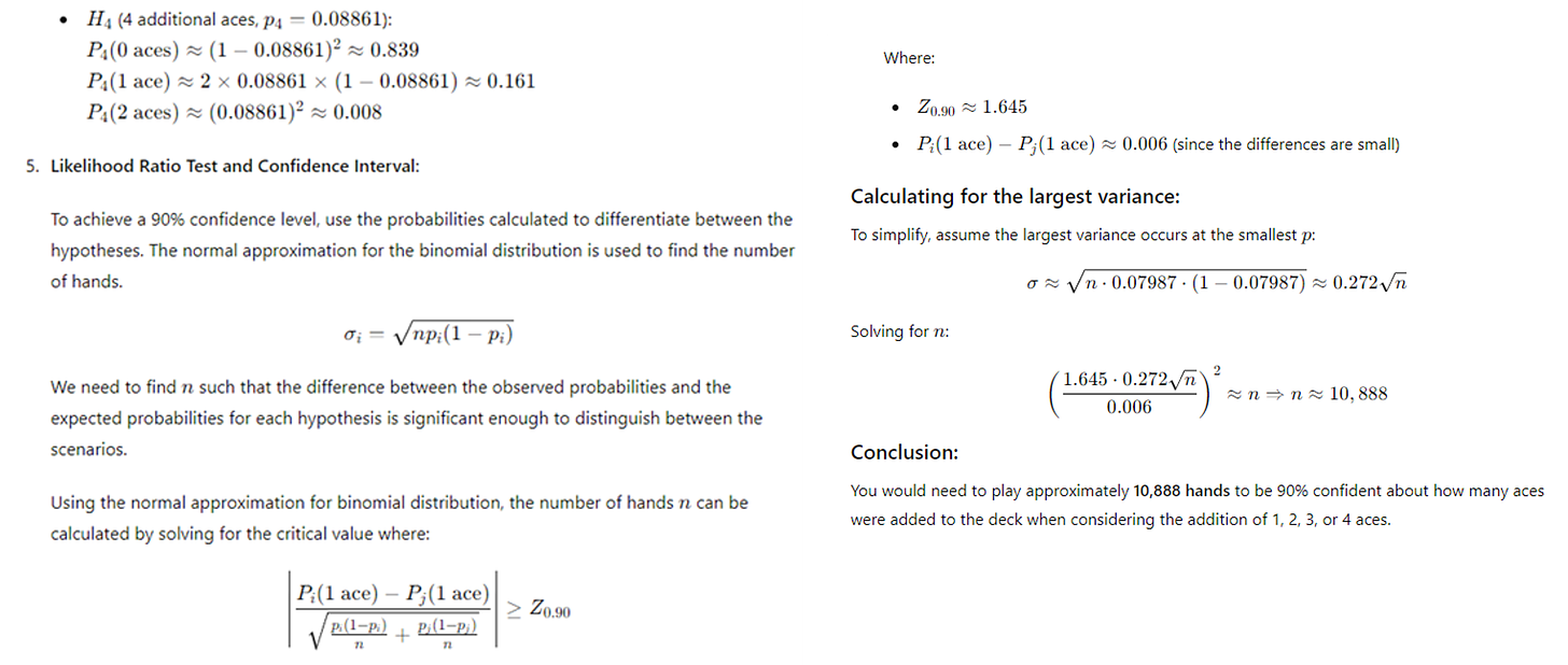
Let’s imagine that I may have added 1, 2, 3, or 4 aces to the combined deck (we could name each RCP 2.6, 4.5, 6.0, and 8.5). How many two-card hands would we have to play before we reach the IPCC threshold for detection of change, i.e., 90% confidence about how many aces have been added?

The answer is a big number — 10,888 hands!⁶

This helps to explain why some climate experts wish to abandon the IPCC’s framework for detection and attribution, and just assume that metrics of extreme weather have changed. Detection of change with high confidence in highly variable time series is challenging!

Let’s assume four added aces. Then we implement an “ace mitigation policy” and remove two of them. How many two-card hands would we have to play before we reach the IPCC threshold for detection of change in two-card hands?

The answer = 8,203 hands.

What about removing 3 of the 4 aces?

2,211 hands.

The large difference in “time of emergence” between removing two versus three aces helps us to understand the climate community’s affinity toward extreme scenarios — Extreme counterfactual baselines makes it easier to detect projected change due to policy — though detection is still challenging even using extreme scenarios as counterfactual baselines.

The IPCC explains that the effects of successful mitigation policy would first be detected in carbon dioxide concentrations, then decades later in average global temperatures, and for other variables not until later this century, at best:

Among global quantities, emergence of the response to differing CO2 emissions – representing differences between low- and high-emissions scenarios – is first expected to arise in global mean CO2 concentrations, about 10 years after emissions pathways have started diverging . . .

Taking internal variability explicitly into account, Tebaldi and Friedlingstein (2013) and Samset et al. (2020) found emergence of mitigation benefits in GSAT [global surface air temperature] changes about 25–30 years after RCP2.6 emissions diverge from the higher-emissions trajectories in RCP4.5 and RCP8.5 . . .

. . . the response of many other climate quantities to mitigation would be largely masked by internal variability during the near term, especially on the regional scale (high confidence). The mitigation benefits for these quantities would emerge only later during the 21st century (high confidence).

In plain English this means that the effects of climate mitigation policies on the weather you experience in your lifetime would not be detectable, even if you are born in 2024. This explains why for most variables associated with extreme events the IPCC’s projection of the “time of emergence” of a climate change or climate mitigation signal is so far into the future.

None of this means that human-caused climate change is not real or important. What it does mean is that those politicians, scientists, and journalists who are promising to stop or slow down extreme weather and its impacts through energy policy are peddling misinformation.

There are plenty of excellent reasons why accelerating the century-long trend in global decarbonization makes sense. Stopping extreme weather is not among these reasons. Climate advocacy would be more effective if it were grounded in real benefits of decarbonization to people, and not in misleading fantasies of controlling the weather.

Comments welcomed! THB is reader supported and reader engaged. If you value what you read here, please share and subscribe — Your support is what makes the THB community possible.

1. There are many different scenarios, many different models, and many different realizations — so this IPCC example is highly simplified.

2. This also tells us that many of the published studies showing changes in this or that variable are little more than parlor games in the absence of formal approaches to detection and attribution that consider climate variability.

3. The IPCC actually employs 10 different “reference periods” as shown below from the AR6 Technical Summary.

4. All calculations in this post courtesy ChatGPT.

5. This is the equivalent of adding (or subtracting) one ace from the combined deck over 80 years.

6. Here is the math: